library(openxlsx) # Datos de Excel
library(raster)   # Datos raster
library(sf) # Datos vectorialesLectura y escritura
Importación de librerías
1. Archivos CSV
a. Importación de archivos CSV
data_CSV <- read.csv(file = 'data/iris.csv',
                     sep = ',')
head(data_CSV, 3)
SepalLength SepalWidth PetalLength PetalWidth Name
1 5.1 3.5 1.4 0.2 Iris-setosa
2 4.9 3.0 1.4 0.2 Iris-setosa
3 4.7 3.2 1.3 0.2 Iris-setosaclass(data_CSV)[1] "data.frame"b. Exportación de archivos CSV
write.csv(x = data_CSV,
          file = 'data_CSV.csv',
row.names = FALSE) write.csv(x = data_CSV,
file = 'data_CSV.csv',
row.names = FALSE) 2. Archivos TXT
a. Importación de archivos TXT
La función read.table de R puede leer tanto archivos CSV como TXT.
data_TXT <- read.table(file = 'data/iris.txt',
                       sep = ',',
                       header = TRUE)
head(data_TXT, 3)
SepalLength SepalWidth PetalLength PetalWidth Name
1 5.1 3.5 1.4 0.2 Iris-setosa
2 4.9 3.0 1.4 0.2 Iris-setosa
3 4.7 3.2 1.3 0.2 Iris-setosaclass(data_TXT)[1] "data.frame"b. Exportación de archivos TXT
write.table(x = data_TXT,
            file = 'data_TXT.txt',
            sep = ',',
            row.names = FALSE)
3. Archivos de Excel
a. Importación de archivos Excel
Los archivos de Excel se leen por medio de la librería openxlsx
data_XLSX <- read.xlsx(xlsxFile = 'data/iris.xlsx')
head(data_XLSX, 3)
SepalLength SepalWidth PetalLength PetalWidth Name
1 5.1 3.5 1.4 0.2 Iris-setosa
2 4.9 3.0 1.4 0.2 Iris-setosa
3 4.7 3.2 1.3 0.2 Iris-setosaclass(data_XLSX)[1] "data.frame"b. Exportación de archivos Excel
write.xlsx(x = data_XLSX,
           file = "data_XLSX.xlsx")
4. Archivos raster
a. Importación de archivos raster
Los archivos raster se pueden leer por medio de la libreria raster
data_Raster <- raster(x = 'data/PERU_dem.tif')
data_Raster
class : RasterLayer
dimensions : 2232, 1560, 3481920 (nrow, ncol, ncell)
resolution : 0.008333333, 0.008333333 (x, y)
extent : -81.5, -68.5, -18.5, 0.1 (xmin, xmax, ymin, ymax)
crs : +proj=longlat +datum=WGS84 +no_defs
source : PERU_dem.tif
names : PERU_dem
values : -25, 6547 (min, max)plot(data_Raster,
main="DEM Peru")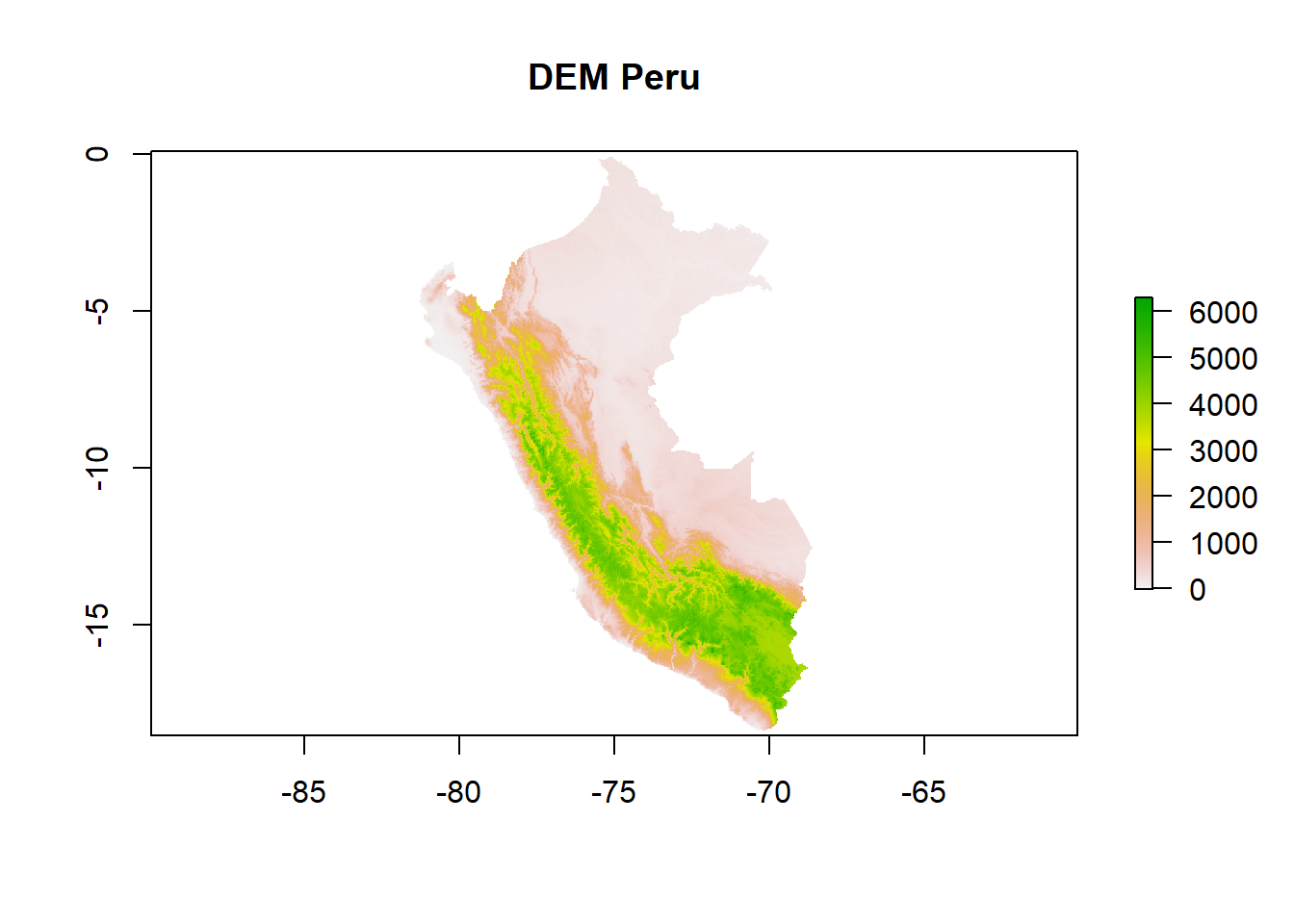
b. Exportación de archivos raster
writeRaster(x = data_Raster,
            filename = "dem.tif")
5. Archivos vectoriales
a. Importación de archivos vectoriales
data_SHP <- read_sf(dsn = 'data/SHP/Departamentos_Peru.shp')
head(data_SHP, n=3)
Simple feature collection with 3 features and 9 fields
Geometry type: MULTIPOLYGON
Dimension: XY
Bounding box: xmin: -78.71218 ymin: -14.84273 xmax: -72.0512 ymax: -2.986125
Geodetic CRS: WGS 84
# A tibble: 3 × 10
CCDD NOMBDEP POBTOTAL DENSIDAD POBMASCU POBFEMEN POBURBANA POBRURAL
<chr> <chr> <dbl> <dbl> <dbl> <dbl> <dbl> <dbl>
1 01 AMAZONAS 417365 1980. 211439 205926 205980 211385
2 02 ANCASH 1139115 7396. 565184 573931 806068 333047
3 03 APURIMAC 424259 2696. 211338 212921 243350 180909
# ℹ 2 more variables: EDAD_PROME <dbl>, geometry <MULTIPOLYGON [°]>plot(st_geometry(data_SHP),
col = rainbow(24),
border="black",
lwd=0.1,
bg = "skyblue",
axes=TRUE,
main="Mapa del Perú")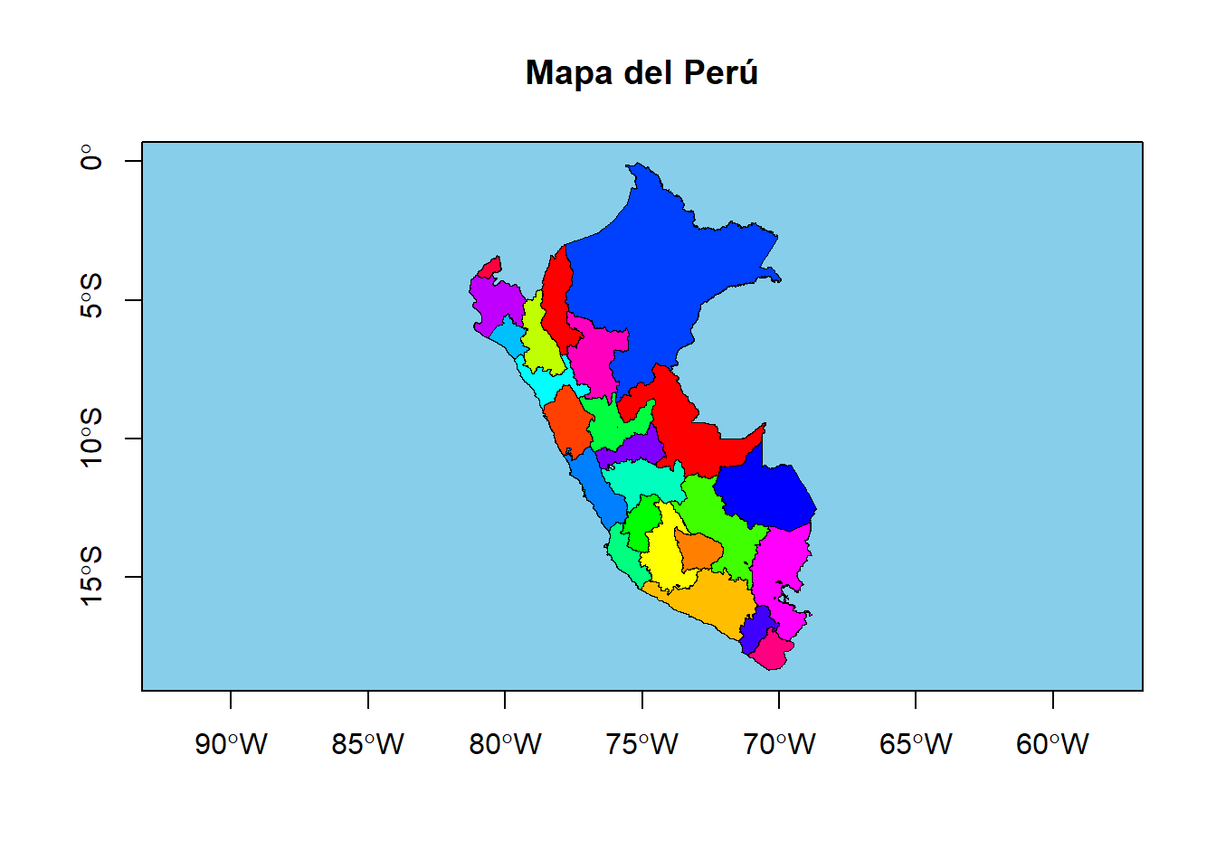
b. Exportación de archivos vectoriales
st_write(obj = data_SHP,
         dsn = "data_SHP.shp",
         driver = "ESRI Shapefile")