library(sf)
library(tidyverse) Libreria SF
1. Importación
Importacion de librerías
Importación de los archivos vectoriales en formato shapefile
poligonos <- read_sf('data/Poligonos.shp')
lineas <- read_sf('data/Lineas.shp')
puntos <- read_sf('data/Puntos.shp')
Los datos vectoriales importados son del tipo SF
class(poligonos)[1] "sf" "tbl_df" "tbl" "data.frame"class(lineas)[1] "sf" "tbl_df" "tbl" "data.frame"class(puntos)[1] "sf" "tbl_df" "tbl" "data.frame"a. Polígono
poligonosSimple feature collection with 4 features and 4 fields
Geometry type: POLYGON
Dimension: XY
Bounding box: xmin: 674144.9 ymin: 8468463 xmax: 683605.9 ymax: 8473273
Projected CRS: WGS 84 / UTM zone 18S
# A tibble: 4 × 5
Id Objeto Area Perimetro geometry
<dbl> <chr> <dbl> <dbl> <POLYGON [m]>
1 1 Triangulo 3.56 8.60 ((677159.6 8470790, 678593.3 8473273, 680027…
2 2 Cuadrado 4 8 ((674144.9 8471479, 676144.9 8471479, 676144…
3 3 Rectangulo 7.10 12.4 ((674968 8469981, 679647.6 8469981, 679647.6…
4 4 Hexagono 6.14 9.23 ((680942.4 8469776, 680942.4 8471314, 682274…plot(poligonos["Objeto"])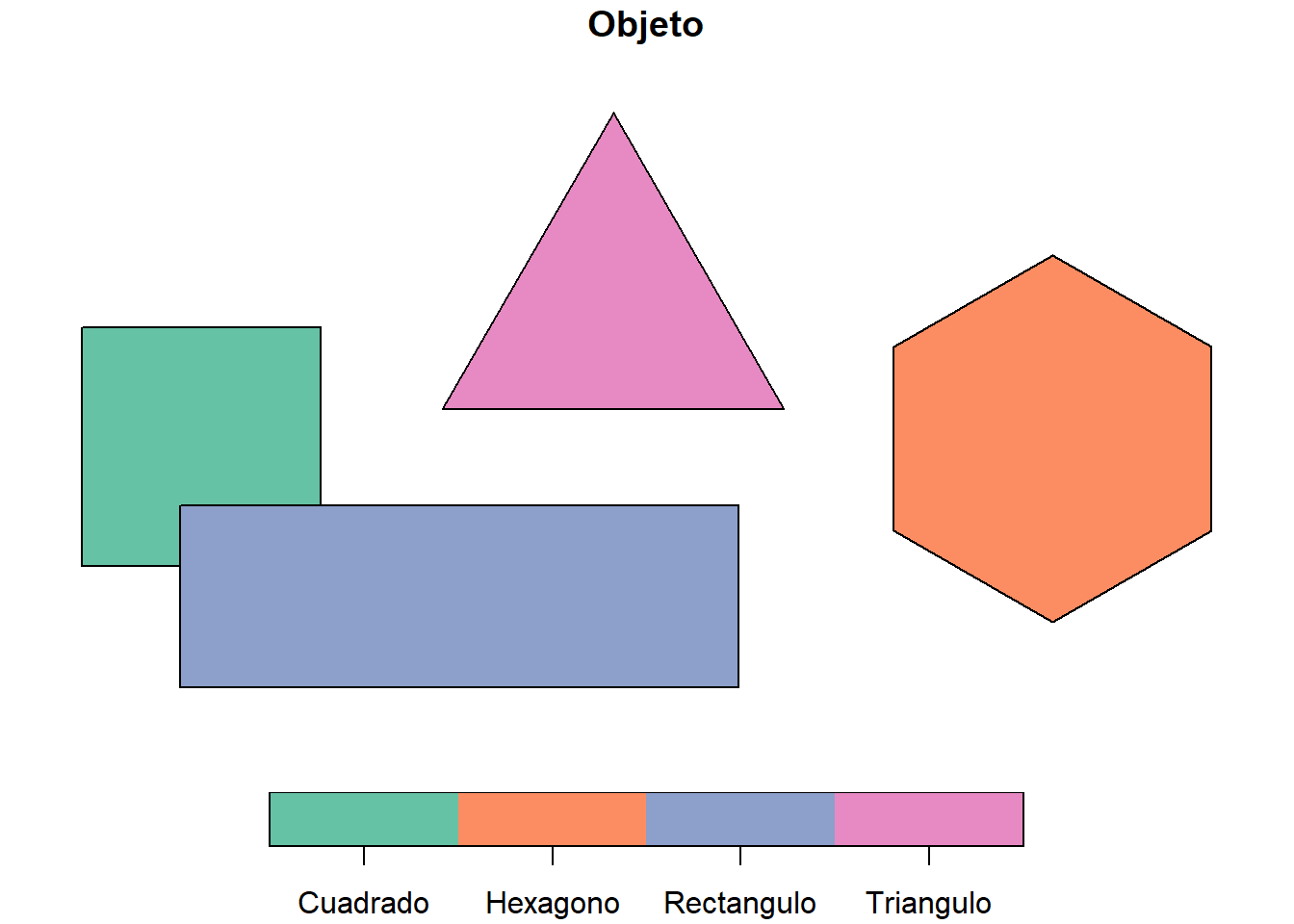
b. Línea
lineasSimple feature collection with 4 features and 3 fields
Geometry type: LINESTRING
Dimension: XY
Bounding box: xmin: 672984.3 ymin: 8468543 xmax: 683554.9 ymax: 8475568
Projected CRS: WGS 84 / UTM zone 18S
# A tibble: 4 × 4
Id Objeto Longitud geometry
<dbl> <chr> <dbl> <LINESTRING [m]>
1 1 Linea 1 7.51 (672984.3 8473006, 677316.8 8473006, 676303.6 8473591,…
2 2 Linea 2 5.46 (676779.3 8470448, 680330 8470448, 680330 8468543)
3 3 Linea 3 3.40 (680786 8471947, 679086.5 8474891)
4 4 Linea 4 7.49 (681242.1 8472631, 681242.1 8474064, 683554.9 8474064,…plot(lineas["Objeto"], lwd = 3)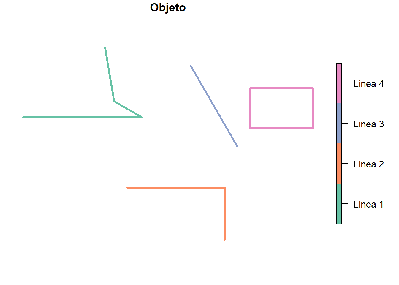
c. Punto
puntosSimple feature collection with 10 features and 2 fields
Geometry type: POINT
Dimension: XY
Bounding box: xmin: 673391.5 ymin: 8469145 xmax: 682577.7 ymax: 8474406
Projected CRS: WGS 84 / UTM zone 18S
# A tibble: 10 × 3
Id Objeto geometry
<dbl> <chr> <POINT [m]>
1 1 Punto 1 (674922.5 8472370)
2 2 Punto 2 (676795.6 8470986)
3 3 Punto 3 (677528.5 8474406)
4 4 Punto 4 (679206.1 8471247)
5 5 Punto 5 (673391.5 8470302)
6 6 Punto 6 (680004.2 8469145)
7 7 Punto 7 (682577.7 8473348)
8 8 Punto 8 (678505.8 8472322)
9 9 Punto 9 (675346 8469748)
10 10 Punto 10 (678424.3 8469162)plot(puntos["Objeto"], pch = 19)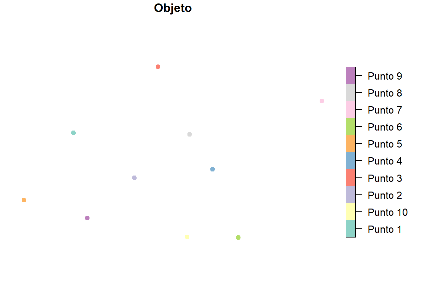
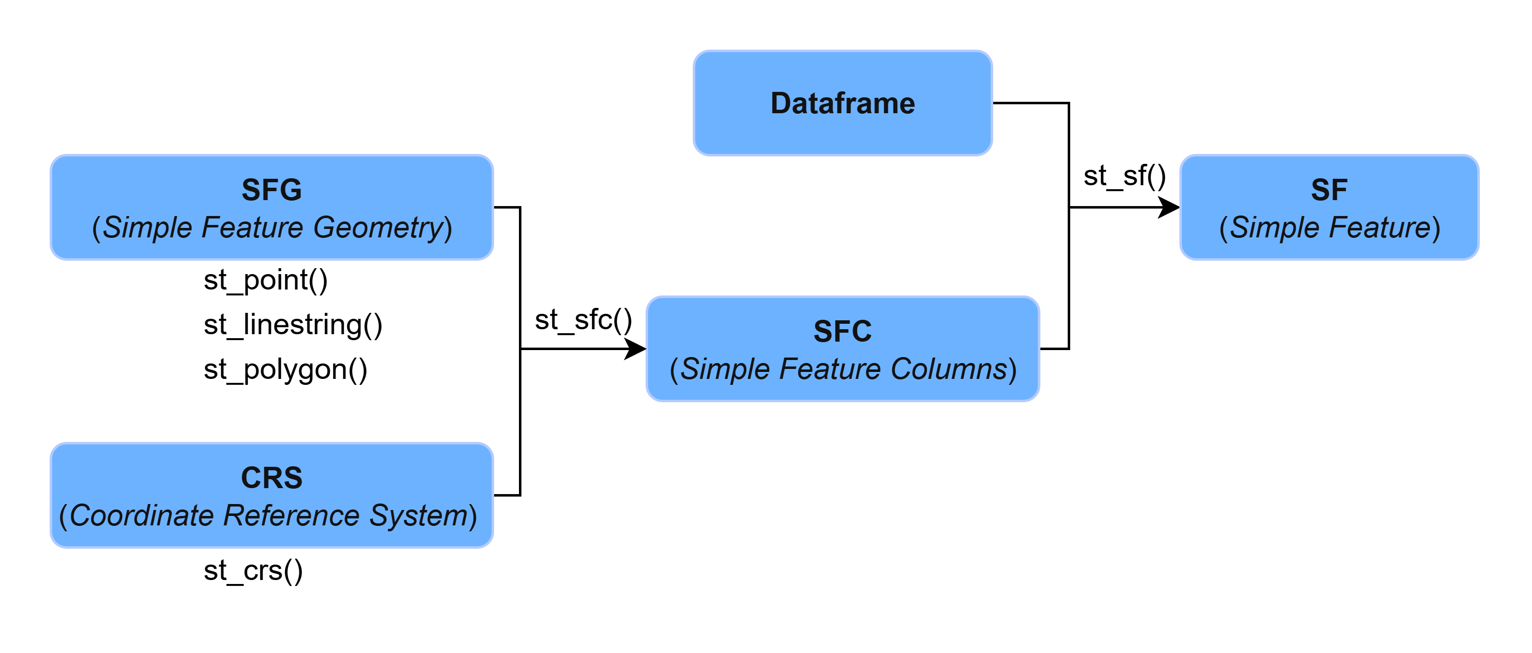
2. Elementos
Un objeto SF esta comformado por los siguientes elementos:
- Objeto Dataframe
- Objeto SFC
- Objeto SFG
- Objeto CRS
a. Objeto Dataframe
El Dataframe representa la tabla de atributos del archivo shapefile.
ST_SET_GEOMETRY
df <- st_set_geometry(poligonos, NULL)
df
# A tibble: 4 × 4
Id Objeto Area Perimetro
* <dbl> <chr> <dbl> <dbl>
1 1 Triangulo 3.56 8.60
2 2 Cuadrado 4 8
3 3 Rectangulo 7.10 12.4
4 4 Hexagono 6.14 9.23class(df)[1] "tbl_df" "tbl" "data.frame"b. Objeto SFC
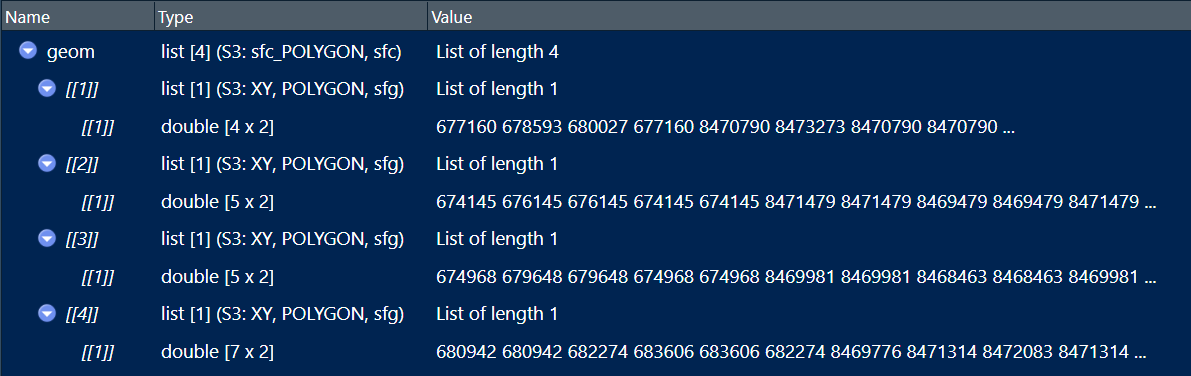
El objeto SFC (Simple Feature Column) representa la geometría de un dato vectorial, el cual contiene las coordenadas de los vértices asi como su sistema de referencia (CRS).
Se puede acceder a través de la funcion st_geometry(poligonos) o poligonos$geometry.
ST_GEOMETRY
geom <- st_geometry(poligonos)
geom
Geometry set for 4 features
Geometry type: POLYGON
Dimension: XY
Bounding box: xmin: 674144.9 ymin: 8468463 xmax: 683605.9 ymax: 8473273
Projected CRS: WGS 84 / UTM zone 18Sclass(geom)[1] "sfc_POLYGON" "sfc" La información del objeto SFC esta estructurado de la siguiente manera:
c. Objeto SFG
El objeto SFG (Simple Feature Geometry) representa la forma del tipo de geometria (puntos, lineas, poligonos) el cual esta formado por un conjunto de coordenadas.
Por ejemplo, el segundo elemento del dato poligono es una geometría de forma cuadrada.
geom[[2]]class(geom[[2]])[1] "XY" "POLYGON" "sfg" plot(geom[[2]])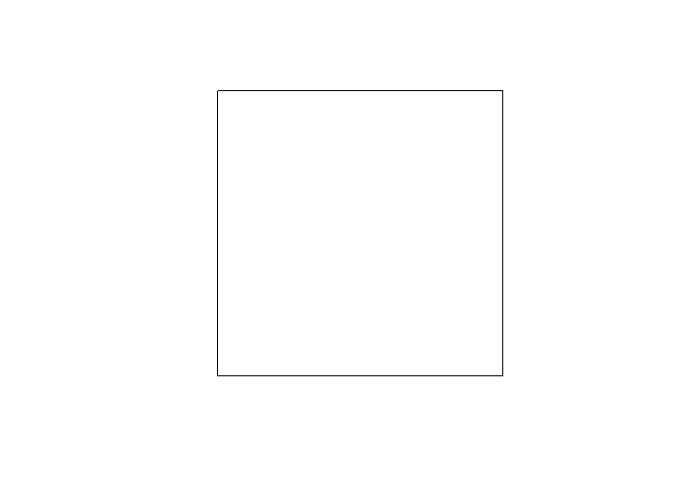
Las coordenadas del cuadrado son sus vértices que se encuentran ordenadas en una matriz en donde la primera columna es la coordenada X y la segunda la coordenada Y.
geom[[2]][[1]] [,1] [,2]
[1,] 674144.9 8471479
[2,] 676144.9 8471479
[3,] 676144.9 8469479
[4,] 674144.9 8469479
[5,] 674144.9 8471479class(geom[[2]][[1]])[1] "matrix" "array" d. Objeto CRS
El objeto CRS contiene el Sistema de Coordenadas de Referencia (CRS).
ST_CRS
st_crs(geom)Coordinate Reference System:
User input: WGS 84 / UTM zone 18S
wkt:
PROJCRS["WGS 84 / UTM zone 18S",
BASEGEOGCRS["WGS 84",
DATUM["World Geodetic System 1984",
ELLIPSOID["WGS 84",6378137,298.257223563,
LENGTHUNIT["metre",1]]],
PRIMEM["Greenwich",0,
ANGLEUNIT["degree",0.0174532925199433]],
ID["EPSG",4326]],
CONVERSION["UTM zone 18S",
METHOD["Transverse Mercator",
ID["EPSG",9807]],
PARAMETER["Latitude of natural origin",0,
ANGLEUNIT["Degree",0.0174532925199433],
ID["EPSG",8801]],
PARAMETER["Longitude of natural origin",-75,
ANGLEUNIT["Degree",0.0174532925199433],
ID["EPSG",8802]],
PARAMETER["Scale factor at natural origin",0.9996,
SCALEUNIT["unity",1],
ID["EPSG",8805]],
PARAMETER["False easting",500000,
LENGTHUNIT["metre",1],
ID["EPSG",8806]],
PARAMETER["False northing",10000000,
LENGTHUNIT["metre",1],
ID["EPSG",8807]]],
CS[Cartesian,2],
AXIS["(E)",east,
ORDER[1],
LENGTHUNIT["metre",1]],
AXIS["(N)",north,
ORDER[2],
LENGTHUNIT["metre",1]],
ID["EPSG",32718]]